stats: The R Base Package

R標準の統計解析パッケージ

• CRAN: https://stat.ethz.ch/R-manual/R-devel/library/stats/html/00Index.html

> library(stats)

バージョン: 3.2.3

Distributions

確率分布

> # dbeta
> # dbinom
> # dcauchy
> # ...

Lognormal / dlnorm / plnorm / qlnorm / rlnorm

対数正規分布

Arguments

• x, q
• p
• meanlog, sdlog
• log, log.p
• lower.tail

> rlnorm(n = 10)

 [1] 4.1484730 2.3108145 0.3768001 0.1954081 0.4252516 0.2927458 1.2176975
 [8] 0.1893988 1.3688176 0.4578168

acf / pacf / ccf

自己相関のプロット

> acf(lh)
> acf(lh, type = "covariance")
> pacf(lh)

aggregate

要約統計量の算出

> iris %>% aggregate(. ~ Species, data = ., mean)

     Species Sepal.Length Sepal.Width Petal.Length Petal.Width
1     setosa        5.006       3.428        1.462       0.246
2 versicolor        5.936       2.770        4.260       1.326
3  virginica        6.588       2.974        5.552       2.026

ave

> data(warpbreaks)
> ave(warpbreaks$breaks, warpbreaks$wool)

 [1] 31.03704 31.03704 31.03704 31.03704 31.03704 31.03704 31.03704
 [8] 31.03704 31.03704 31.03704 31.03704 31.03704 31.03704 31.03704
[15] 31.03704 31.03704 31.03704 31.03704 31.03704 31.03704 31.03704
[22] 31.03704 31.03704 31.03704 31.03704 31.03704 31.03704 25.25926
[29] 25.25926 25.25926 25.25926 25.25926 25.25926 25.25926 25.25926
[36] 25.25926 25.25926 25.25926 25.25926 25.25926 25.25926 25.25926
[43] 25.25926 25.25926 25.25926 25.25926 25.25926 25.25926 25.25926
[50] 25.25926 25.25926 25.25926 25.25926 25.25926

> iris %$% ave(Sepal.Length, Species)

  [1] 5.006 5.006 5.006 5.006 5.006 5.006 5.006 5.006 5.006 5.006 5.006
 [12] 5.006 5.006 5.006 5.006 5.006 5.006 5.006 5.006 5.006 5.006 5.006
 [23] 5.006 5.006 5.006 5.006 5.006 5.006 5.006 5.006 5.006 5.006 5.006
 [34] 5.006 5.006 5.006 5.006 5.006 5.006 5.006 5.006 5.006 5.006 5.006
 [45] 5.006 5.006 5.006 5.006 5.006 5.006 5.936 5.936 5.936 5.936 5.936
 [56] 5.936 5.936 5.936 5.936 5.936 5.936 5.936 5.936 5.936 5.936 5.936
 [67] 5.936 5.936 5.936 5.936 5.936 5.936 5.936 5.936 5.936 5.936 5.936
 [78] 5.936 5.936 5.936 5.936 5.936 5.936 5.936 5.936 5.936 5.936 5.936
 [89] 5.936 5.936 5.936 5.936 5.936 5.936 5.936 5.936 5.936 5.936 5.936
[100] 5.936 6.588 6.588 6.588 6.588 6.588 6.588 6.588 6.588 6.588 6.588
[111] 6.588 6.588 6.588 6.588 6.588 6.588 6.588 6.588 6.588 6.588 6.588
[122] 6.588 6.588 6.588 6.588 6.588 6.588 6.588 6.588 6.588 6.588 6.588
[133] 6.588 6.588 6.588 6.588 6.588 6.588 6.588 6.588 6.588 6.588 6.588
[144] 6.588 6.588 6.588 6.588 6.588 6.588 6.588

complete.cases

欠損値の確認

> complete.cases(c(1, 2, NA, 4))

[1]  TRUE  TRUE FALSE  TRUE

decompose

> x <- c(-50, 175, 149, 214, 247, 237, 225, 329, 729, 809,
+        530, 489, 540, 457, 195, 176, 337, 239, 128, 102, 232, 429, 3,
+        98, 43, -141, -77, -13, 125, 361, -45, 184) %>% 
+   ts(start = c(1951, 1), end = c(1958, 4), frequency = 4)
> decompose(x)

$x
     Qtr1 Qtr2 Qtr3 Qtr4
1951  -50  175  149  214
1952  247  237  225  329
1953  729  809  530  489
1954  540  457  195  176
1955  337  239  128  102
1956  232  429    3   98
1957   43 -141  -77  -13
1958  125  361  -45  184

$seasonal
          Qtr1      Qtr2      Qtr3      Qtr4
1951  62.45982  86.17411 -88.37946 -60.25446
1952  62.45982  86.17411 -88.37946 -60.25446
1953  62.45982  86.17411 -88.37946 -60.25446
1954  62.45982  86.17411 -88.37946 -60.25446
1955  62.45982  86.17411 -88.37946 -60.25446
1956  62.45982  86.17411 -88.37946 -60.25446
1957  62.45982  86.17411 -88.37946 -60.25446
1958  62.45982  86.17411 -88.37946 -60.25446

$trend
        Qtr1    Qtr2    Qtr3    Qtr4
1951      NA      NA 159.125 204.000
1952 221.250 245.125 319.750 451.500
1953 561.125 619.250 615.625 548.000
1954 462.125 381.125 316.625 264.000
1955 228.375 210.750 188.375 199.000
1956 207.125 191.000 166.875  72.000
1957  -9.250 -33.125 -36.750  36.250
1958 103.000 131.625      NA      NA

$random
            Qtr1        Qtr2        Qtr3        Qtr4
1951          NA          NA   78.254464   70.254464
1952  -36.709821  -94.299107   -6.370536  -62.245536
1953  105.415179  103.575893    2.754464    1.254464
1954   15.415179  -10.299107  -33.245536  -27.745536
1955   46.165179  -57.924107   28.004464  -36.745536
1956  -37.584821  151.825893  -75.495536   86.254464
1957  -10.209821 -194.049107   48.129464   11.004464
1958  -40.459821  143.200893          NA          NA

$figure
[1]  62.45982  86.17411 -88.37946 -60.25446

$type
[1] "additive"

attr(,"class")
[1] "decomposed.ts"

dist

距離行列

Arguments

• x
• method... euclidean, maximum, manhattan, canberra, binary, minkowski
• diag... 出力オプション
• upper... 出力オプション
• p
• m
• digits, justify
• right
• ...

> x <- matrix(rnorm(100), nrow = 5)
> dist(x)

         1        2        3        4
2 5.535243                           
3 6.339792 7.941767                  
4 7.089858 7.070399 4.346966         
5 5.811479 7.041772 5.518783 6.457818

> dist(x, diag = TRUE)

         1        2        3        4        5
1 0.000000                                    
2 5.535243 0.000000                           
3 6.339792 7.941767 0.000000                  
4 7.089858 7.070399 4.346966 0.000000         
5 5.811479 7.041772 5.518783 6.457818 0.000000

> dist(x, upper = TRUE)

         1        2        3        4        5
1          5.535243 6.339792 7.089858 5.811479
2 5.535243          7.941767 7.070399 7.041772
3 6.339792 7.941767          4.346966 5.518783
4 7.089858 7.070399 4.346966          6.457818
5 5.811479 7.041772 5.518783 6.457818

family

モデリングのための確率分布オブジェクト

Arguments

• link
• variance
• object
• ...

filter

時系列データのフィルタリング

Arguments

• x
• filter
• method
• sides
• circular

> x <- 1:100
> filter(x, rep(1, 3))

Time Series:
Start = 1 
End = 100 
Frequency = 1 
  [1]  NA   6   9  12  15  18  21  24  27  30  33  36  39  42  45  48  51
 [18]  54  57  60  63  66  69  72  75  78  81  84  87  90  93  96  99 102
 [35] 105 108 111 114 117 120 123 126 129 132 135 138 141 144 147 150 153
 [52] 156 159 162 165 168 171 174 177 180 183 186 189 192 195 198 201 204
 [69] 207 210 213 216 219 222 225 228 231 234 237 240 243 246 249 252 255
 [86] 258 261 264 267 270 273 276 279 282 285 288 291 294 297  NA

> filter(x, rep(1, 3), sides = 1, circular = TRUE)

Time Series:
Start = 1 
End = 100 
Frequency = 1 
  [1] 200 103   6   9  12  15  18  21  24  27  30  33  36  39  42  45  48
 [18]  51  54  57  60  63  66  69  72  75  78  81  84  87  90  93  96  99
 [35] 102 105 108 111 114 117 120 123 126 129 132 135 138 141 144 147 150
 [52] 153 156 159 162 165 168 171 174 177 180 183 186 189 192 195 198 201
 [69] 204 207 210 213 216 219 222 225 228 231 234 237 240 243 246 249 252
 [86] 255 258 261 264 267 270 273 276 279 282 285 288 291 294 297

hclust

階層クラスタリング

Arguments

• d... distクラスオブジェクト
• method... ward.D, ward.D2, single, complete, average, mcquitty, median, centroid
• members
• x
• hang
• check
• labels
• axes, frame.plot, ann
• main, sub, xlab, ylab
• ...

> dist(USArrests) %>% hclust(method = "ave")

Call:
hclust(d = ., method = "ave")

Cluster method   : average 
Distance         : euclidean 
Number of objects: 50

lag

時系列の差分

Arguments

• x
• k
• ...

> lag(x = ldeaths, k = 12)

      Jan  Feb  Mar  Apr  May  Jun  Jul  Aug  Sep  Oct  Nov  Dec
1973 3035 2552 2704 2554 2014 1655 1721 1524 1596 2074 2199 2512
1974 2933 2889 2938 2497 1870 1726 1607 1545 1396 1787 2076 2837
1975 2787 3891 3179 2011 1636 1580 1489 1300 1356 1653 2013 2823
1976 3102 2294 2385 2444 1748 1554 1498 1361 1346 1564 1640 2293
1977 2815 3137 2679 1969 1870 1633 1529 1366 1357 1570 1535 2491
1978 3084 2605 2573 2143 1693 1504 1461 1354 1333 1492 1781 1915

margin.table

> matrix(1:4, 2) %>% {
+   print(margin.table(., 1))
+   margin.table(., 2)
+ }

[1] 4 6

[1] 3 7

na.fail / na.omit / na.exclude / na.pass

オブジェクト内の欠損処理

> DT <- data.frame(x = c(1, 2, 3), y = c(0, 10, NA))
> DT %>% {
+   print(na.omit(.))
+   print(na.pass(.))
+ }

  x  y
1 1  0
2 2 10
  x  y
1 1  0
2 2 10
3 3 NA

p.adjust

P値の補正

> set.seed(123)
> x <- rnorm(50, mean = c(rep(0, 25), rep(3, 25)))
> p <- 2*pnorm(sort(-abs(x)))
> 
> round(p, 3)

 [1] 0.000 0.000 0.000 0.000 0.000 0.000 0.000 0.000 0.000 0.000 0.001
[12] 0.002 0.003 0.004 0.005 0.007 0.007 0.009 0.009 0.011 0.021 0.049
[23] 0.061 0.063 0.074 0.083 0.086 0.119 0.189 0.206 0.221 0.286 0.305
[34] 0.466 0.483 0.492 0.532 0.575 0.578 0.619 0.636 0.645 0.656 0.689
[45] 0.719 0.818 0.827 0.897 0.912 0.944

> round(p.adjust(p), 3)

 [1] 0.000 0.001 0.001 0.005 0.005 0.006 0.006 0.007 0.009 0.016 0.024
[12] 0.063 0.125 0.131 0.189 0.239 0.240 0.291 0.301 0.350 0.635 1.000
[23] 1.000 1.000 1.000 1.000 1.000 1.000 1.000 1.000 1.000 1.000 1.000
[34] 1.000 1.000 1.000 1.000 1.000 1.000 1.000 1.000 1.000 1.000 1.000
[45] 1.000 1.000 1.000 1.000 1.000 1.000

> round(p.adjust(p, "BH"), 3)

 [1] 0.000 0.000 0.000 0.001 0.001 0.001 0.001 0.001 0.001 0.002 0.003
[12] 0.007 0.013 0.013 0.017 0.021 0.021 0.024 0.025 0.028 0.050 0.112
[23] 0.130 0.130 0.148 0.159 0.160 0.213 0.326 0.343 0.356 0.446 0.462
[34] 0.684 0.684 0.684 0.719 0.741 0.741 0.763 0.763 0.763 0.763 0.782
[45] 0.799 0.880 0.880 0.930 0.930 0.944

procomp

主成分分析を実施

Arguments

• formula
• data
• subset
• na.action
• ...
• x
• retx
• center... logical. 中央化（中心移動）の有無
• scale... logical. 標準化の有無
• object
• newdata

spectrum

> spectrum(lh)

start / end

時系列データの始点と終点

> xts::xts(rnorm(21), as.Date((Sys.Date() %>% as.numeric() - 20):Sys.Date() %>% as.numeric(), origin = "1970-01-01")) %>% {
+   start(.) %>% print()
+   end(.)
+ }

[1] "2016-02-16"

[1] "2016-03-07"

> data("presidents")
> presidents %>% {
+   start(.) %>% print()
+   end(.)
+ }

[1] 1945    1

[1] 1974    4

time / cycle/ deltat / frequency

時系列データに関する処理諸々

> time(presidents) %>% as.vector()

  [1] 1945.00 1945.25 1945.50 1945.75 1946.00 1946.25 1946.50 1946.75
  [9] 1947.00 1947.25 1947.50 1947.75 1948.00 1948.25 1948.50 1948.75
 [17] 1949.00 1949.25 1949.50 1949.75 1950.00 1950.25 1950.50 1950.75
 [25] 1951.00 1951.25 1951.50 1951.75 1952.00 1952.25 1952.50 1952.75
 [33] 1953.00 1953.25 1953.50 1953.75 1954.00 1954.25 1954.50 1954.75
 [41] 1955.00 1955.25 1955.50 1955.75 1956.00 1956.25 1956.50 1956.75
 [49] 1957.00 1957.25 1957.50 1957.75 1958.00 1958.25 1958.50 1958.75
 [57] 1959.00 1959.25 1959.50 1959.75 1960.00 1960.25 1960.50 1960.75
 [65] 1961.00 1961.25 1961.50 1961.75 1962.00 1962.25 1962.50 1962.75
 [73] 1963.00 1963.25 1963.50 1963.75 1964.00 1964.25 1964.50 1964.75
 [81] 1965.00 1965.25 1965.50 1965.75 1966.00 1966.25 1966.50 1966.75
 [89] 1967.00 1967.25 1967.50 1967.75 1968.00 1968.25 1968.50 1968.75
 [97] 1969.00 1969.25 1969.50 1969.75 1970.00 1970.25 1970.50 1970.75
[105] 1971.00 1971.25 1971.50 1971.75 1972.00 1972.25 1972.50 1972.75
[113] 1973.00 1973.25 1973.50 1973.75 1974.00 1974.25 1974.50 1974.75

> cycle(presidents)

     Qtr1 Qtr2 Qtr3 Qtr4
1945    1    2    3    4
1946    1    2    3    4
1947    1    2    3    4
1948    1    2    3    4
1949    1    2    3    4
1950    1    2    3    4
1951    1    2    3    4
1952    1    2    3    4
1953    1    2    3    4
1954    1    2    3    4
1955    1    2    3    4
1956    1    2    3    4
1957    1    2    3    4
1958    1    2    3    4
1959    1    2    3    4
1960    1    2    3    4
1961    1    2    3    4
1962    1    2    3    4
1963    1    2    3    4
1964    1    2    3    4
1965    1    2    3    4
1966    1    2    3    4
1967    1    2    3    4
1968    1    2    3    4
1969    1    2    3    4
1970    1    2    3    4
1971    1    2    3    4
1972    1    2    3    4
1973    1    2    3    4
1974    1    2    3    4

> deltat(presidents)

[1] 0.25

> frequency(presidents)

[1] 4

ts

時系列オブジェクト

Arguments

• data
• start
• end
• frequency
• deltat
• ts.eps
• class
• names
• x
• ...

> ts(1:10, frequency = 4, start = c(1959, 2))

     Qtr1 Qtr2 Qtr3 Qtr4
1959         1    2    3
1960    4    5    6    7
1961    8    9   10

Value

• sdev... 主成分の標準偏差
• rotation... 主成分負荷量（各変数と主成分との相関係数）
• x
• center, scale

> library(vegan)

Loading required package: permute

Attaching package: 'permute'

The following object is masked from 'package:devtools':

    check

Loading required package: lattice

This is vegan 2.3-4

> data(dune)
> tmp <- prcomp(dune, scale = TRUE)
> tmp

Standard deviations:
 [1] 2.651876e+00 2.235468e+00 1.885408e+00 1.626053e+00 1.462502e+00
 [6] 1.325825e+00 1.215869e+00 1.147346e+00 1.052556e+00 8.994324e-01
[11] 8.632887e-01 8.346228e-01 7.582115e-01 5.982967e-01 4.717356e-01
[16] 4.687690e-01 3.882168e-01 3.631904e-01 2.519873e-01 2.196148e-16

Rotation:
                  PC1          PC2          PC3          PC4         PC5
Achimill  0.277358149 -0.015906183 -0.171540078 -0.049173592 -0.29797708
Agrostol -0.270446458  0.225338171  0.075149364 -0.022996313  0.02558700
Airaprae  0.001618847 -0.334422632  0.274278753  0.056419555 -0.21157505
Alopgeni -0.099368966  0.262715304  0.202867708  0.183634250  0.07939982
Anthodor  0.202286085 -0.252994352 -0.025027518  0.149016455 -0.25727867
Bellpere  0.201572477  0.127576066  0.038861550 -0.322454771 -0.07154160
Bromhord  0.225274286  0.118823565 -0.002994863 -0.251045921 -0.22298470
Chenalbu -0.054616149  0.119088370  0.135179981  0.232444003 -0.12138149
Cirsarve  0.016649960  0.149380662  0.193439742 -0.189189359  0.05836970
Comapalu -0.161477760 -0.039960081 -0.187024484 -0.106012285 -0.19183468
Eleopalu -0.293597121 -0.006473954 -0.227685384 -0.094858485 -0.04635077
Elymrepe  0.109724080  0.240308038  0.133618192 -0.093621154 -0.08257644
Empenigr -0.006634467 -0.306810069  0.291414519  0.041757498 -0.08967878
Hyporadi  0.017519532 -0.352770478  0.288137299  0.004269798 -0.03521201
Juncarti -0.238810633  0.054362038 -0.104288726  0.005407353  0.12006764
Juncbufo -0.030874269  0.168783055  0.160848821  0.394627384  0.05976745
Lolipere  0.260781049  0.126992599 -0.053228671 -0.173046076  0.19908008
Planlanc  0.260637241 -0.115975258 -0.252281165  0.152008787  0.12508002
Poaprat   0.247586440  0.211405188  0.045967251 -0.147978053  0.18606513
Poatriv   0.147625073  0.320567091  0.098901591  0.195193384 -0.13875194
Ranuflam -0.306240477  0.007882711 -0.168936684 -0.028939692 -0.05685098
Rumeacet  0.177246450  0.004371686 -0.205222489  0.406962363  0.05580819
Sagiproc -0.037114076  0.070055086  0.402043149  0.083191067  0.18822893
Salirepe -0.115885992 -0.237949108  0.034692521 -0.100795686  0.16147267
Scorautu  0.170911118 -0.232081941  0.135559337 -0.107874951  0.16122343
Trifprat  0.179727680 -0.045658643 -0.260817422  0.328898976  0.06476554
Trifrepe  0.167398084  0.019578344 -0.113457105 -0.022272789 -0.08044923
Vicilath  0.112386371 -0.106027466 -0.028724352 -0.238177831  0.38835725
Bracruta -0.025688498 -0.141949026 -0.141161217  0.090465605  0.51332296
Callcusp -0.244915366 -0.037979317 -0.222350635 -0.113087021 -0.13890022
                  PC6          PC7           PC8          PC9         PC10
Achimill -0.018250222 -0.006282728 -0.1465146630 -0.037072033 -0.284943943
Agrostol  0.186756604  0.245082868  0.0123098484 -0.119510658 -0.110920492
Airaprae  0.096422424 -0.097712511  0.0321399888 -0.009575434 -0.099636156
Alopgeni -0.105946895  0.020135820 -0.0824459661  0.190755977 -0.332376870
Anthodor  0.156125796  0.026640693 -0.0500822271 -0.115352982 -0.235971913
Bellpere  0.085903724  0.187617173 -0.2832554823  0.139865201  0.126977572
Bromhord  0.099278861  0.281830918 -0.1759418372 -0.012395382 -0.215272689
Chenalbu -0.354866757  0.111081984 -0.2457657313 -0.442523896  0.230253188
Cirsarve  0.418278378  0.321366302  0.1896615933 -0.317577712  0.082926161
Comapalu -0.140848501  0.213691628  0.4385138707  0.162039456  0.272304254
Eleopalu  0.086146760  0.039331789 -0.0006513118  0.039218528 -0.335830173
Elymrepe  0.262309219 -0.245075057  0.0238913356  0.339835808  0.352362019
Empenigr  0.093431268  0.077015555 -0.0416727213  0.185013217 -0.019670023
Hyporadi -0.004373535 -0.049490532  0.0919817016 -0.001399784 -0.103591182
Juncarti  0.154461344 -0.179380327 -0.2079525280  0.271134136 -0.283072280
Juncbufo -0.201014256  0.039793136 -0.0083079686  0.182621410  0.031942060
Lolipere  0.018960837 -0.180667416  0.1327932031 -0.077020674 -0.113576629
Planlanc  0.044506375  0.056964592 -0.0185270317 -0.214586350  0.016949100
Poaprat  -0.033908359 -0.229590251 -0.0138181427 -0.004776205 -0.023703719
Poatriv  -0.028641057  0.103937114 -0.2547465226  0.011586367 -0.038789045
Ranuflam -0.042350839  0.090057291 -0.2759871539 -0.125750626  0.001195093
Rumeacet  0.246487606  0.113785393  0.0366406873  0.134230105  0.114249032
Sagiproc  0.115864362  0.311970978  0.1808234119 -0.042954530 -0.140063426
Salirepe  0.118664904  0.045789547 -0.5063249251  0.042911714  0.335199480
Scorautu -0.173373768  0.251032453 -0.1852370018  0.228971454  0.077604381
Trifprat  0.232524328  0.128553835  0.0437890155 -0.042611817  0.089272402
Trifrepe -0.322607335  0.422132017  0.1215698753  0.383096915 -0.067705602
Vicilath -0.352398143  0.040430177  0.0618260529 -0.177126252 -0.118331138
Bracruta  0.159976508  0.205823892 -0.0964632149  0.102689199 -0.085332107
Callcusp  0.018570846  0.167200631 -0.0181969123  0.034626421  0.067508897
                 PC11         PC12         PC13         PC14         PC15
Achimill  0.132717925  0.134230514 -0.034529992  0.216182453 -0.141401817
Agrostol -0.059618860 -0.073683574 -0.023668258 -0.123235118 -0.106634349
Airaprae -0.019070127 -0.058358107  0.012396331  0.006629187  0.077238090
Alopgeni  0.039952489 -0.472711933 -0.065874698  0.056133072  0.142673465
Anthodor  0.099085859  0.039405527  0.030439268 -0.182295662 -0.191244567
Bellpere  0.191229646 -0.339813778  0.178784646 -0.145988631 -0.020153703
Bromhord  0.109494416  0.244018820  0.037703343  0.079868176 -0.018373727
Chenalbu -0.227060023  0.018287239  0.171677291 -0.175868511 -0.279195670
Cirsarve -0.003959815  0.141735155  0.001321334  0.049219524  0.036375284
Comapalu -0.051236512  0.049521631  0.419309406  0.122054623 -0.083871507
Eleopalu -0.131378144 -0.080553382  0.131165765 -0.207537309  0.007388714
Elymrepe  0.007174943  0.106204727 -0.030839977 -0.418387219 -0.195258305
Empenigr -0.304035391 -0.042476542 -0.027675462 -0.013779008 -0.351380876
Hyporadi -0.161835620  0.006085387 -0.045001999 -0.226512749  0.026476252
Juncarti -0.135408677  0.460006428  0.263053866 -0.143056615 -0.011814909
Juncbufo  0.331943950  0.383004314 -0.131204452  0.096142350 -0.059442194
Lolipere -0.399550594  0.009446008 -0.192536364  0.230441982 -0.122499231
Planlanc  0.112734237  0.045729471  0.043171048 -0.234799012  0.262590230
Poaprat  -0.325080178  0.091586125 -0.011846325  0.019010072  0.047744134
Poatriv  -0.209438657 -0.058924074  0.084029572 -0.135860829  0.013058855
Ranuflam -0.253468364  0.167283523  0.028297656  0.048388895  0.121361026
Rumeacet -0.017167126  0.032043329 -0.022347327 -0.179664647  0.114973393
Sagiproc  0.010890721  0.227060385 -0.066484762  0.028308217  0.124594706
Salirepe  0.042105059  0.100015813 -0.222850655  0.290392613 -0.071386194
Scorautu -0.181281016  0.048423771  0.228628199 -0.063119924  0.505549613
Trifprat -0.316843001 -0.089080821 -0.027087807  0.076188887  0.007168476
Trifrepe -0.198256965  0.071632853 -0.243172011  0.018039774 -0.180390197
Vicilath  0.148055454  0.120910330 -0.060677691 -0.428538696 -0.180520174
Bracruta  0.122374527 -0.190949281  0.161598801  0.073266522 -0.429555487
Callcusp -0.045372709 -0.035110432 -0.635088337 -0.283642351  0.111397731
                 PC16         PC17         PC18        PC19         PC20
Achimill  0.006319455 -0.250624910  0.130057211 -0.15259224 -0.280840132
Agrostol  0.129552488  0.220228162  0.032570554 -0.33376824  0.117562664
Airaprae  0.210143799  0.075340772  0.313245566 -0.17648404 -0.028419294
Alopgeni  0.141347045  0.067080980 -0.209999376 -0.17097107  0.077234388
Anthodor  0.389496778  0.221157627 -0.313756777  0.05751084  0.086145893
Bellpere  0.094710988  0.044306606  0.001176329  0.06773279 -0.233103744
Bromhord -0.374362864  0.041343305 -0.053691688 -0.14594158  0.305384469
Chenalbu  0.006875299 -0.091678747  0.173724870  0.09615198 -0.086869927
Cirsarve  0.143093017  0.062180079  0.221579806  0.00292687  0.004781978
Comapalu  0.024471933  0.243764018 -0.231073572 -0.23547941 -0.203407714
Eleopalu -0.316846051  0.038250547  0.153274202  0.26832548 -0.338905630
Elymrepe -0.003495925 -0.192734275 -0.038247140 -0.14099381  0.058019662
Empenigr -0.341052828  0.242487410 -0.163670390  0.27686627  0.252889870
Hyporadi -0.091888742 -0.083198813  0.020109210 -0.44286040 -0.372522205
Juncarti  0.235944145  0.009026855  0.102938841  0.02591653  0.001586611
Juncbufo -0.191629105  0.329604360  0.162314310 -0.18263770 -0.071387835
Lolipere -0.160510751  0.048846040 -0.219803850 -0.21507924 -0.173345126
Planlanc -0.056120436  0.405994596 -0.104807822  0.05804021 -0.114153392
Poaprat   0.213962048  0.415537482  0.145898300  0.13921121 -0.091198432
Poatriv  -0.136171340  0.082075532 -0.069242868 -0.10994713 -0.207521475
Ranuflam  0.119804645 -0.138589298 -0.347714187 -0.20643369  0.135135821
Rumeacet -0.053875908 -0.155850682 -0.220366196  0.02634990 -0.124352068
Sagiproc  0.031989882 -0.272388398 -0.267648595  0.29545079 -0.279033917
Salirepe  0.121935233  0.114820087 -0.173474729 -0.02796627 -0.265406160
Scorautu -0.079587214 -0.030689931  0.151345426 -0.09463241  0.158732103
Trifprat  0.022440237 -0.167076686  0.220113547 -0.15845608  0.210115585
Trifrepe  0.366480663 -0.060442109  0.127395719  0.15596121 -0.023897121
Vicilath  0.030320179 -0.106893186 -0.142322601 -0.14990616  0.134383490
Bracruta -0.061532092 -0.010759652  0.187268280 -0.13283957 -0.052130439
Callcusp -0.085439050  0.140108877  0.131246343 -0.03698375 -0.057840003

> # plot(tmp)
> # barplot(log(tmp$sdev) ^ 2, names.arg = seq(1:4),
> #         xlab = "component",
> #         ylab = "variance")
> 
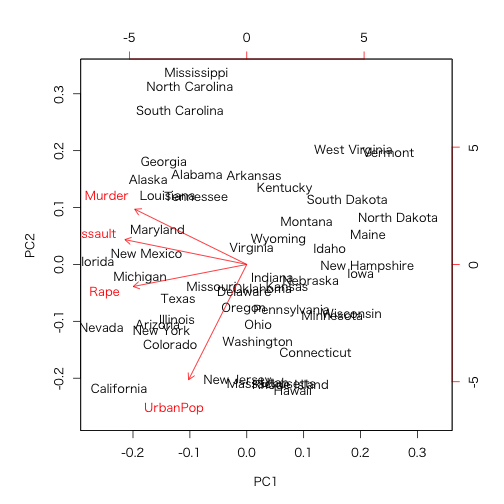
> data(USArrests) # 1973年のアメリカにおける犯罪に関するデータ（犯罪の種類および都市部人口の割合、州）
> prcomp(~ Murder + Assault + Rape, 
+        data = USArrests, 
+        scale = TRUE)

Standard deviations:
[1] 1.5357670 0.6767949 0.4282154

Rotation:
               PC1        PC2        PC3
Murder  -0.5826006  0.5339532 -0.6127565
Assault -0.6079818  0.2140236  0.7645600
Rape    -0.5393836 -0.8179779 -0.1999436

> # plot(prcomp(USArrests))
> summary(prcomp(USArrests, scale = TRUE))

Importance of components:
                          PC1    PC2     PC3     PC4
Standard deviation     1.5749 0.9949 0.59713 0.41645
Proportion of Variance 0.6201 0.2474 0.08914 0.04336
Cumulative Proportion  0.6201 0.8675 0.95664 1.00000

> biplot(prcomp(USArrests, scale = TRUE))

prop.table

割合テーブルの作成

> matrix(1:4, 2) %>% {
+   print(.)
+   prop.table(., 1)
+ }

     [,1] [,2]
[1,]    1    3
[2,]    2    4

          [,1]      [,2]
[1,] 0.2500000 0.7500000
[2,] 0.3333333 0.6666667

terms

> ctl <- c(4.17,5.58,5.18,6.11,4.50,4.61,5.17,4.53,5.33,5.14)
> trt <- c(4.81,4.17,4.41,3.59,5.87,3.83,6.03,4.89,4.32,4.69)
> group <- gl(2, 10, 20, labels = c("Ctl","Trt"))
> weight <- c(ctl, trt)
> 
> lm(weight ~ group) %>% terms()

weight ~ group
attr(,"variables")
list(weight, group)
attr(,"factors")
       group
weight     0
group      1
attr(,"term.labels")
[1] "group"
attr(,"order")
[1] 1
attr(,"intercept")
[1] 1
attr(,"response")
[1] 1
attr(,".Environment")
<environment: 0x10c24bd20>
attr(,"predvars")
list(weight, group)
attr(,"dataClasses")
   weight     group 
"numeric"  "factor"

window

時系列データの抽出

Arguments

• x
• start
• end
• frequency, deltat
• extend
• ...
• value

> window(x = presidents,  start = 1960, end = c(1969, 4))

     Qtr1 Qtr2 Qtr3 Qtr4
1960   71   62   61   57
1961   72   83   71   78
1962   79   71   62   74
1963   76   64   62   57
1964   80   73   69   69
1965   71   64   69   62
1966   63   46   56   44
1967   44   52   38   46
1968   36   49   35   44
1969   59   65   65   56