ggmcmc: Tools for Analyzing MCMC Simulations from Bayesian Inference
MCMCシュミレーション結果の解析ツール
- CRAN: http://cran.r-project.org/web/packages/ggmcmc/index.html
- GitHub: https://github.com/xfim/ggmcmc
- URL: http://xavier-fim.net/packages/ggmcmc
> library(ggmcmc)
Loading required package: dplyr

Attaching package: 'dplyr'

The following object is masked from 'package:sfsmisc':

    last

The following object is masked from 'package:MASS':

    select

The following objects are masked from 'package:stats':

    filter, lag

The following objects are masked from 'package:base':

    intersect, setdiff, setequal, union

Loading required package: tidyr

Attaching package: 'tidyr'

The following object is masked from 'package:coenocliner':

    expand

The following object is masked from 'package:rstan':

    extract

The following object is masked from 'package:Matrix':

    expand

The following object is masked from 'package:magrittr':

    extract

Loading required package: GGally
Warning: replacing previous import by 'grid::arrow' when loading 'GGally'
Warning: replacing previous import by 'grid::unit' when loading 'GGally'
Attaching package: 'GGally'

The following object is masked from 'package:dplyr':

    nasa
> data("radon")
バージョン: 0.7.2
| 関数名 | 概略 |
|---|---|
ac |
Calculate the autocorrelation of a single chain, for a specified amount of lags |
calc_bin |
Calculate binwidths by parameter, based on the total number of bins. |
ci |
Calculate Credible Intervals (wide and narrow). |
get_family |
Subset a ggs object to get only the parameters with a given regular expression. |
ggmcmc |
Wrapper function that creates a single pdf file with all plots that ggmcmc can produce. |
ggs |
Import MCMC samples into a ggs object than can be used by all ggs_* graphical functions. |
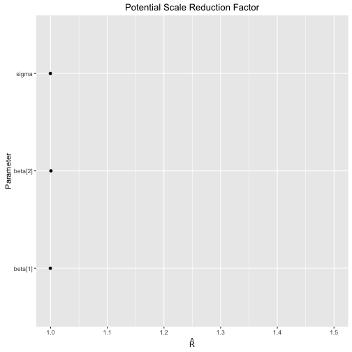
ggs_Rhat |
Dotplot of Potential Scale Reduction Factor (Rhat) |
ggs_autocorrelation |
Plot an autocorrelation matrix |
ggs_caterpillar |
Caterpillar plot with thick and thin CI |
ggs_chain |
Auxiliary function that extracts information from a single chain. |
ggs_compare_partial |
Density plots comparing the distribution of the whole chain with only its last part. |
ggs_crosscorrelation |
Plot the Cross-correlation between-chains |
ggs_density |
Density plots of the chains |
ggs_geweke |
Dotplot of the Geweke diagnostic, the standard Z-score |
ggs_histogram |
Histograms of the paramters. |
ggs_pairs |
Create a plot matrix of posterior simulations |
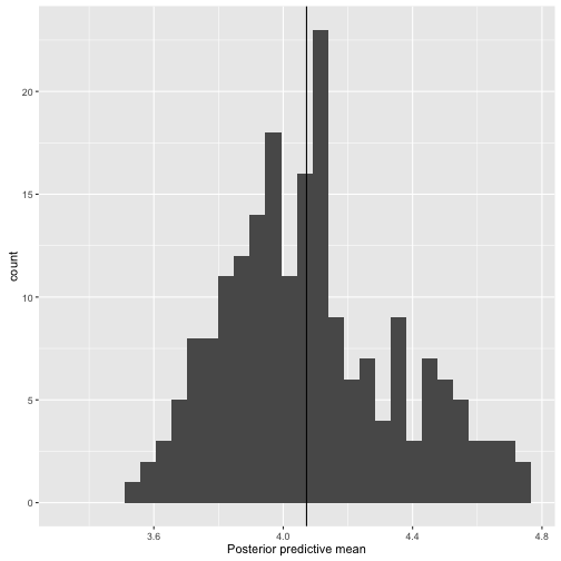
ggs_ppmean |
Posterior predictive plot comparing the outcome mean vs the distribution of the predicted posterior means. |
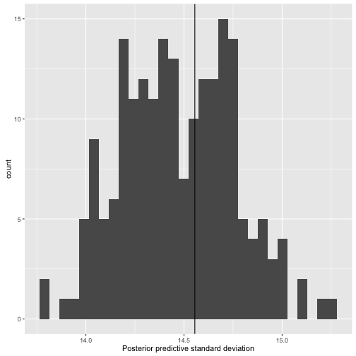
ggs_ppsd |
Posterior predictive plot comparing the outcome standard deviation vs the distribution of the predicted posterior standard deviations. |
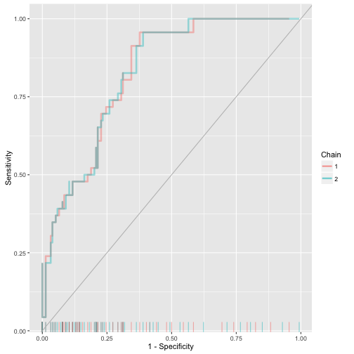
ggs_rocplot |
Receiver-Operator Characteristic (ROC) plot for models with binary outcomes |
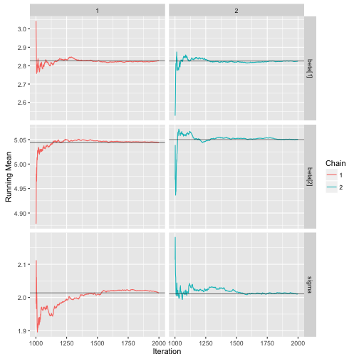
ggs_running |
Running means of the chains |
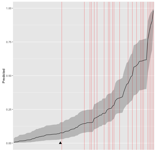
ggs_separation |
Separation plot for models with binary response variables |
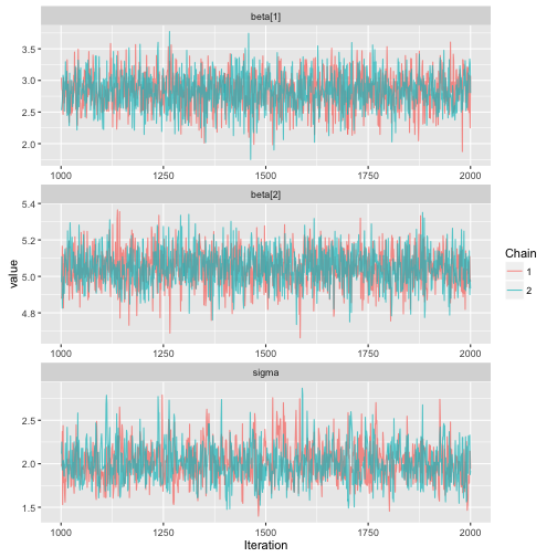
ggs_traceplot |
Traceplot of the chains |
gl_unq |
Generate a factor with unequal number of repetitions. |
radon |
Simulations of the parameters of a hierarchical model using the radon example in Gelman & Hill (2007). |
roc_calc |
Calculate the ROC curve for a set of observed outcomes and predicted probabilities |
s |
Simulations of the parameters of a simple linear regression with fake data. |
s.binary |
Simulations of the parameters of a simple linear regression with fake data. |
s.y.rep |
Simulations of the posterior predictive distribution of a simple linear regression with fake data. |
sde0f |
Spectral Density Estimate at Zero Frequency. |
y |
Values for the observed outcome of a simple linear regression with fake data. |
y.binary |
Values for the observed outcome of a binary logistic regression with fake data. |
ac
自己相関の検証。ggs_autocorretation()で用いられている。
> ac(cumsum(rnorm(10)) / 10, nLags = 5)
  Lag Autocorrelation
1   1       1.0000000
2   2       0.8713890
3   3       0.7159419
4   4       0.8814559
5   5       0.9853668
ci
信用区間の算出
> s %>% ggs() %>% ci() %>%
+   kable()
Error in eval(expr, envir, enclos): object 's' not found
ggmcmc
{ggmcmc}で描画できるすべてのプロットをPDFとして保存
Arguments
- D
- file... 保存するPDFファイル名。初期値は"ggmcmc-output.pdf"
- family
- plot... 描画対象にする関数。文字列として関数名を与える。
- param_page
- width
- height
- simplify_traceplot
- ...
> s %>% ggs() %>%
+   ggmcmc()
> s %>% ggs() %>%
+   ggmcmc(plot = c("ggs_running", "ggs_autocorrelation"))
ggs
MCMC事後サンプルを{ggmcmc}内のggs_*()で利用可能なggsオブジェクト(data.frame, tbl_dfクラス)へ変換。反復回数、チェインの数、パラメータ名、値の列を持つ。
Arguments
- S... samples
- family
- description
- burnin
- par_labels
- inc_warmup
- stan_include_auxiliar
> s %>% ggs() %>% {
+   print(class(.))
+   dplyr::glimpse(.)
+ }
Error in eval(expr, envir, enclos): object 's' not found
> radon$s.radon.short %>% ggs() %>% {
+   print(class(.))
+   dplyr::glimpse(.)
+ }
[1] "tbl_df"     "tbl"        "data.frame"
Observations: 16,000
Variables: 4
$ Iteration (int) 1, 2, 3, 4, 5, 6, 7, 8, 9, 10, 11, 12, 13, 14, 15, 1...
$ Chain     (int) 1, 1, 1, 1, 1, 1, 1, 1, 1, 1, 1, 1, 1, 1, 1, 1, 1, 1...
$ Parameter (fctr) alpha[1], alpha[1], alpha[1], alpha[1], alpha[1], a...
$ value     (dbl) 1.9675268, 1.0572830, 1.1732732, 1.2637594, 1.036500...
ggs_autocorrelation
> data("linear")
> s %>% ggs() %>% ggs_autocorrelation()

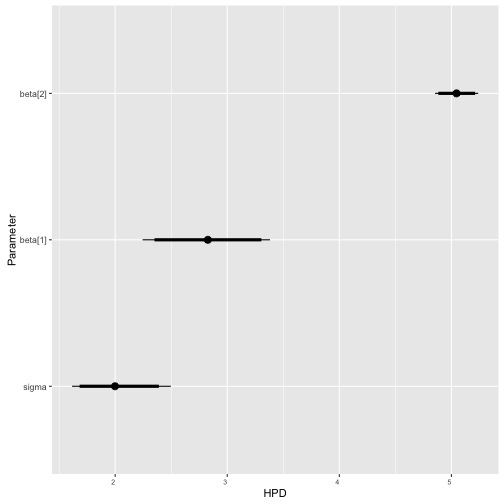
ggs_caterpillar
> data("linear")
> s %>% ggs() %>% ggs_caterpillar()
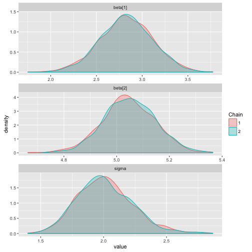
ggs_compare_partial
> data("linear")
> s %>% ggs() %>% ggs_compare_partial()

ggs_crosscorrelation
> data("linear")
> s %>% ggs() %>% ggs_crosscorrelation()

ggs_density
> data("linear")
> s %>% ggs() %>% ggs_density
ggs_geweke
> data("linear")
> s %>% ggs() %>% ggs_geweke()

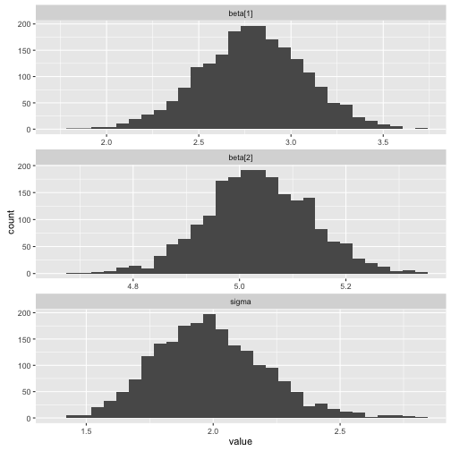
ggs_histogram
> data("linear")
> s %>% ggs() %>% ggs_histogram()
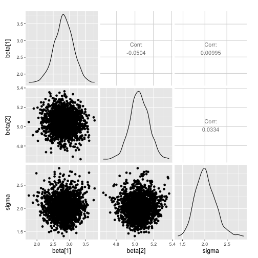
ggs_pairs
> data("linear")
> s %>% ggs() %>% ggs_pairs()
ggs_ppmean
> data("linear")
> s.y.rep %>% ggs() %>% ggs_ppmean(outcome = y)
Error in ggs_ppmean(., outcome = y): The length of the outcome must be equal to the number of Parameters of the ggs object.
ggs_ppsd
> data("linear")
> s.y.rep %>% ggs() %>% ggs_ppsd(outcome = y)
Error in ggs_ppsd(., outcome = y): The length of the outcome must be equal to the number of Parameters of the ggs object.
ggs_rocplot
> data("binary")
> s.binary %>% ggs(family = "mu") %>% ggs_rocplot(outcome = y.binary)
ggs_running
> data("linear")
> s %>% ggs() %>% ggs_running()
ggs_separation
> data("binary")
> s.binary %>% ggs(family = "mu") %>% ggs_separation(outcome = y.binary)
ggs_traceplot
> data("linear")
> s %>% ggs() %>% ggs_traceplot()
ggs_Rhat
> s %>% ggs() %>%
+   ggs_Rhat()
radon
> data("radon")
> radon %>% {
+   print(class(.))
+   print(names(.))
+   str(., max.level = 2)
+ }
[1] "list"
[1] "counties"      "id.county"     "y"             "s.radon"
[5] "s.radon.yhat"  "s.radon.short"
List of 6
 $ counties     :'data.frame':    85 obs. of  4 variables:
  ..$ County     : chr [1:85] "Aitkin" "Anoka" "Becker" "Beltrami" ...
  ..$ id.county  : num [1:85] 1 2 3 4 5 6 7 8 9 10 ...
  ..$ uranium    : num [1:85] 0.502 0.429 0.893 0.552 0.867 ...
  ..$ ns.location: chr [1:85] "North" "South" "North" "North" ...
 $ id.county    : num [1:919] 1 1 1 1 2 2 2 2 2 2 ...
 $ y            : num [1:919] 0.788 0.788 1.065 0 1.131 ...
 $ s.radon      :List of 2
  ..$ : mcmc [1:100, 1:175] 1.186 1.119 1.034 0.969 1.282 ...
  .. ..- attr(*, "dimnames")=List of 2
  .. ..- attr(*, "mcpar")= num [1:3] 10020 12000 20
  ..$ : mcmc [1:100, 1:175] 1.399 0.844 1.044 1.014 1.162 ...
  .. ..- attr(*, "dimnames")=List of 2
  .. ..- attr(*, "mcpar")= num [1:3] 10020 12000 20
  ..- attr(*, "class")= chr "mcmc.list"
 $ s.radon.yhat :List of 2
  ..$ : mcmc [1:10, 1:919] 0.807 0.597 0.111 0.374 0.29 ...
  .. ..- attr(*, "dimnames")=List of 2
  .. ..- attr(*, "mcpar")= num [1:3] 32100 33000 100
  ..$ : mcmc [1:10, 1:919] 0.78984 0.32841 0.35366 -0.00246 0.39972 ...
  .. ..- attr(*, "dimnames")=List of 2
  .. ..- attr(*, "mcpar")= num [1:3] 32100 33000 100
  ..- attr(*, "class")= chr "mcmc.list"
 $ s.radon.short:List of 2
  ..$ : mcmc [1:2000, 1:4] 1.97 1.06 1.17 1.26 1.04 ...
  .. ..- attr(*, "dimnames")=List of 2
  .. ..- attr(*, "mcpar")= num [1:3] 12010 32000 10
  ..$ : mcmc [1:2000, 1:4] 0.929 1.521 1.441 1.164 1.238 ...
  .. ..- attr(*, "dimnames")=List of 2
  .. ..- attr(*, "mcpar")= num [1:3] 12010 32000 10
  ..- attr(*, "class")= chr "mcmc.list"
s
模擬データによる単回帰を行った推定結果。mcmc.listクラスオブジェクト
> s %>% {
+   print(class(.))
+   str(., max.level = 2)
+ }
[1] "mcmc.list"
List of 2
 $ : mcmc [1:1000, 1:3] 3.04 2.85 2.85 2.58 2.46 ...
  ..- attr(*, "dimnames")=List of 2
  ..- attr(*, "mcpar")= num [1:3] 1001 2000 1
 $ : mcmc [1:1000, 1:3] 2.53 2.59 2.67 2.81 3.08 ...
  ..- attr(*, "dimnames")=List of 2
  ..- attr(*, "mcpar")= num [1:3] 1001 2000 1
 - attr(*, "class")= chr "mcmc.list"
s.binary
> s.binary %>% {
+   print(class(.))
+   str(., max.level = 2)
+ }
[1] "mcmc.list"
List of 2
 $ : mcmc [1:100, 1:102] 0.01361 0.01663 0.00308 0.00167 0.06182 ...
  ..- attr(*, "dimnames")=List of 2
  ..- attr(*, "mcpar")= num [1:3] 1010 2000 10
 $ : mcmc [1:100, 1:102] 0.04958 0.00532 0.01521 0.00817 0.00462 ...
  ..- attr(*, "dimnames")=List of 2
  ..- attr(*, "mcpar")= num [1:3] 1010 2000 10
 - attr(*, "class")= chr "mcmc.list"
s.y.rep
> s.y.rep %>% {
+   print(class(.))
+   str(., max.level = 2)
+ }
[1] "mcmc.list"
List of 2
 $ : mcmc [1:200, 1:50] -20.8 -21.9 -23.1 -19.3 -21.5 ...
  ..- attr(*, "dimnames")=List of 2
  ..- attr(*, "mcpar")= num [1:3] 2201 2400 1
 $ : mcmc [1:200, 1:50] -25.1 -18.9 -22.3 -21 -17.9 ...
  ..- attr(*, "dimnames")=List of 2
  ..- attr(*, "mcpar")= num [1:3] 2201 2400 1
 - attr(*, "class")= chr "mcmc.list"